Figure 1. The mosaiced plant root is shown in the upper panel, and registered velocity profile along its medial axis in the lower panel. The velocity is relative to the base of the plant root. The corresponding 2D velocity fields used to derive the profile is shown in Figure 2.

REFERENCING SOFTWARE

RootflowRT was written by Hai Jiang and Prof. K. Palaniappan, University of Missouri-Columbia, in collaboration with Prof. Tobias I. Baskin, University of Massachusetts-Amherst. The executable code is freeware; however, in any publications that result from your using it, we ask that you send one of us a reprint, and cite the following references: van der Weele CM, Jiang H, Palaniappan KK, Ivanov VB, Palaniappan K, Baskin TI (2003) A new algorithm for computational image analysis of deformable motion at high spatial and temporal resolution applied to root growth: Roughly uniform elongation in the meristem and also, after an abrupt acceleration, in the elongation zone. Plant Physiology, 132:1138-1148. Jiang HS, Palaniappan K, Baskin TI (2003) A combined matching and tensor method to obtain high fidelity velocity fields from image sequences of the non-rigid motion of plant root growth In MH Hamza ed, IASTED International Conference on Biomedical Engineering, BioMED 2003, ACTA Press, Calgary, Canada, In press.

RootflowRT is under continuous development. Please refer to our web page for the latest version, additional information, and community resources for measuring root growth.
K. Palaniappan palani@cecs.missouri.edu
Tobias Baskin baskin@bio.umass.edu
 
SOFTWARE OVERVIEW

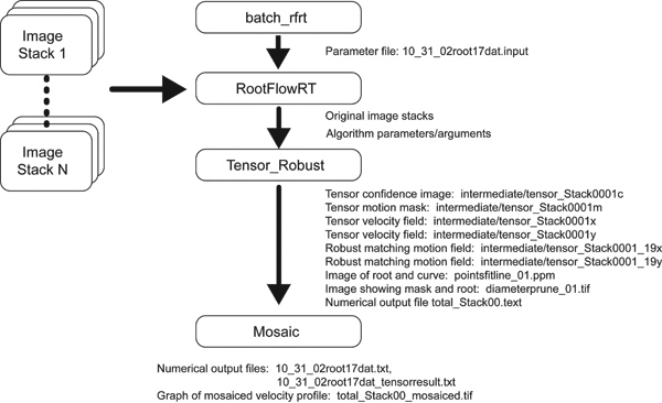
RootflowRT is a package to estimate the spatial velocity profile of plant roots. A velocity profile arises from the expansion (growth) of the elements of the root, and quantification of the velocity profile is sufficient to characterize growth fully. In principle, expansion is three-dimensional, however the software works in two dimensions only, estimating velocity in the plane perpendicular to the imaging axis (focal plane). Roots that undulate in and out of the focal plane are not suitable for analysis at present. Velocity is a vector quantity with a rate and a direction. In view of the fact that the longitudinal axis of the root provides a native axis, velocities are reported parallel and perpendicular to the local tangent to root's midline. The velocity estimation is done on an image volume obtained by capturing a set of 9 images (frames) of the growing root with the same time interval between each frame. Typical time intervals are between 2 to 30 seconds. Velocity estimation uses a structure-tensor method followed by a robust-matching method. Details are provided in the above references, our web page, or by request from us. Both methods rely on the gray level sub-structure (i.e. texture) within the root image. Because elongation is typically of chief interest, the numerical velocity profiles are created by averaging velocity the locus of values perpendicular to each point of the root's midline. The midline can be obtained either algorithmically by the software or can be manually specified by the user. The latter method is very useful for complex roots with many root hairs or other incidental features of the image that make automatic root segmentation more error prone and prevent the program from being 100% successful. To pick midline points, obtain the coordinates of points near the left and right edges of the root, and if the root is bent, then include one or two additional points along the root. Input images must be in either TIFF or PPM format and are typically 640 pixels by 480 pixels and 8 bits per pixel. Support for larger image sizes such as 1280 x 1024, as well as higher gray level quantization resolution of 12 bits per pixel is being added to the software. Each set of 9 images (or frames) is called a stack and the software expects the default filenames of, tiff/stack####frame####, where tiff is the subdirectory name and the # symbol represents one numeric digit and there is a space after the word Frame. Hence up to 9999 stacks each with 9999 frames can be accommodated using this naming scheme; however, the software currently handles up to 99 stacks. In addition to the input image sequences, an input text file is required to specify various parameters for the algorithm. As output, for each segment, the software produces a set of images to show intermediate results and tabulates data for each segment, and for the complete profile produces two sets of tabulated results and a graph. Since the root is long and thin, and larger than the field of view of the microscope for typical resolutions, a set of stacks (or segments) must be obtained, which when mosaiced together span the growth zone. Overlaps between stacks should be about 20 % of the field of view. RootflowRT calculates the velocity profile for each segment and mosaics them together for a complete profile. Presently, two kinds of mosaic can be handled. In the simplest way, the user takes a 10^th image after the 9 in the stack of a highly textured background. The background image file name must be specified by convention as stack####back0001. The focus can be changed to capture the background image, but not the x, y stage position. The software will then mosaic the profiles from each stack by finding the overlap between background images which should have some distinct textural components for the algorithm to produce reliable results. Alternatively, if the user can translate the stage by a specific distance, the software can mosaic the profiles from this information and background images do not need to be obtained. The complete profile is also transformed so that the quiescent center (or root tip) is the origin (i.e., spatial coordinate of zero, velocity of zero). This is the natural frame of reference for the root. The velocity is transformed by averaging values in the vicinity of the tip and subtracting the measured values from these. This can create negative values in places in the profile. For transforming the distance coordinate, the movement of the tip between stacks is accounted for using a steady state growth model with constant tip velocity.
 
INSTALLATION

RootflowRT was developed on SGI workstations under IRIX 6.5 and has been ported to Windows(98, 2000, NT), Mac OSX, and Linux(RedHat). The software is written in ANSI C. This software can be installed into ~username/bin or system wide, as long as the user's command path includes the command directory with the executable programs. For MS Windows, the user can download cygwin from http://www.cygwin.com to emulate the Unix environment, following the Windows Version Readme to install the Windows version.
 
WORKING ENVIRONMENT

Before running the software, the user needs to create a working directory to manage the imagery acquired from the video microscope and the plethora of outputs produced by RootflowRT. The user can choose any name, accepted by the operating system, for the working directory. The working directory contains four sub-directories, pgm, intermediate, curve and tiff. The original root image sequences are expected by default to be in the sub-directory tiff. RootflowRT can also read input image sequences in the PPM format if the images are placed in the pgm sub-directory. The default name of the root images are tiff/stack####frame#### such as tiff/stack0001frame0001. Note that the input image stack consists of a set of 9 separate files, with frame 5 being the center frame. In addition to the image sequences, the user also needs to provide parameter values for the run. Although this data can be entered manually as the program runs or as command line input to the batch programs, it is generally more convenient to organize the user responses into a single input specification file that can be read by the program as needed using the Unix file redirection feature. The format of the input file is given next.
 
INPUT FILE SPECIFICATION

The software will ask a series of questions, and the answers can be saved into an input file. The lines of the input file contain either general parameters (such as the camera calibration to convert pixels to microns), specific parameters such as the number of segments for the root, and switches for certain choices of how the software runs. The syntax of this file is rigid since it replaces manual entry by the user and a sample file is given below. Following that is a set of definitions or explanations for each line. Sample Input Data File:
0
1
7
1.3
2
400
10 37 28
10 41 13
10 43 07
10 44 55
10 46 38
10 48 34
10 50 17
stack1
0 339, 208 289, 636 255
dlr 176 166
stack2
0 340, 193 287, 415 259, 636 216
dlr 171 162
stack3
0 393, 283 287, 634 191
dlr 174 166
stack4
0 414, 636 141
dlr 177 158
stack5
0 396, 231 288, 638 73
dlr 188 166
stack6
0 355, 218 320, 491 231, 638 160
dlr 162 181
stack7
171 317, 637 255
dlr 162 181
endm
10
447 286
10_31_02root17dat.txt
 
  Explanation of Input File Parameters: Note that the format for these lines is the same whether they are in the input file or entered manually in response to prompts from the software. Note also that all spatial coordinates are entered assuming that the origin (0,0) is in the bottom left corner.

-----------------------------------------------------------------------------------------------------------------
0 | Direction of growth: 0=right to left, 1=left to right.
1 | Order of segments: < 0 if first stack is tip, 1 if base>
7 | Number of stacks.
1.3 | Calibration. In this example, 1 um = 1.3 pixel.
2   | Mosaic method, 1=from background image; 2=from camera motion
400 | Amount of camera motion in microns; leave a blank line if
      mosaic method is 1 ie from background image information.
10 37 28 | Time of frame five for stack 1
10 41 13 | Time of frame five for stack 2
10 43 07 | Time of frame five for stack 3
10 44 55 | Time of frame five for stack 4
10 46 38 | Time of frame five for stack 5
10 48 34 | Time of frame five for stack 6
10 50 17 | Time of frame five for stack 7
             [ the above 7 lines provide a time for each
             stack in the run, format is hours min sec]
stack1   | Defines stacks for geometry input.
0 339, 208 289, 636 255 | Pair-wise points (x,y) defining the midline.
dlr 176 166             | Root diameter in pixels near the left and right
                          end of the center image.
stack2                           |[Geometry input is optional. To omit
0 340, 193 287, 415 259, 636 216 |for a stack omit the three lines for
dlr 171 162 | that stack.]
stack3
0 393, 283 287, 634 191
dlr 174 166
stack4
0 414, 636 141
dlr 177 158
stack5
0 396, 231 288, 638 73
dlr 188 166
stack6
0 355, 218 320, 491 231, 638 160
dlr 162 181
stack7
171 317, 637 255
dlr 162 181
endm | Defines the end of geometry input.
10 | Time interval between consecutive frames, in seconds.
447 286 | Coordinates of the mosaic velocity profile origin, in
          pixels. Can be the quiescent center, the root cap-root
          junction, or the extreme tip of the root.
10_31_02root17dat.txt | File name for final numerical output.
----------------------------------------------------------------------------------------------------------------

If the user does not specify the geometry input for one stack, by omitting the lines for stack 3 in the input file then the program will generate the medial axis and diameters for stack 3 from the motion mask itself, but will use the user input midline points for the other stacks. If no geometrical information is given then all stacks will be automatically handled by the program.
  Recent Improvement (01/12/2004): The order of the polynomial function to fit the medial axis can be specified in the input file. For each stack, a new line as "type #" can be added, where the number sign '#' specifies the order of the polinomial. Order 1 for line, 2 for quadratic, etc. When the user is not specifying the type of the medial axis, the program will determine the order by itself, such as if there are only two input points for the medial axis, the order is 1 for a line, if there are three points, it is a quadratic curve, etc.
 
OUTPUT FILES The intermediate results are saved in the intermediate and pgm sub-directories (see flowchart below). The pgm sub-directory contains the output from background image analysis if mosaicing method was selected to use background images instead of camera motion. The curve sub-directory contains raster images of the velocity profiles one per stack, one raster image file of the mosaiced velocity profile along the medial axis, total_Stack00_mosaiced.tif, and one file containing information about the mosaicing process combined with intermediate numerical results from pairwise profile concatenation process, total_Stack00.text. Two final numerical result files are generated and saved in the working directory using the file name specified on the last line of the input file, i.e. in the above example, 10_31_02root17dat.txt
10_31_02root17dat_tensorresult.txt The first part of both of these output files contains information about the image sequence stacks and the analysis parameters from the input file. The second part is the mosaiced velocity profile (parallel, perpendicular and total velocities) sampled uniformly along the medial axis, as computed using the combined robust tensor method (10_31_02root17dat.txt) or from the pure structure tensor method (10_31_02root17dat_tensorresult.txt ). For example, using the above input file, the first part of both output files contains the following lines:
# RootflowRT v2.8, Univ of Missouri-Columbia
# The input parameters are:
# 1 <first stack is: the base--> 0; the tip--> 1>
# 7 <total stack number>
# 1.300000 <1 um = 1.300 pixels>
# 2 <mosaicing based on: camera motion --> 2; background --> 1>
# 520 <camera motion, in pixel>
# The time stamps of center frames, from stack 1:
# 10:37:28 10:41:13 10:43:7 10:44:55 10:46:38 10:48:34 10:50:17
# 4480 480 <width/height of total profile image, in pixel>
# 10 <frame time interval, in second>
# 447 286 <cols and rows from QC to upper-left corner, in pixel>
# 10_31_02root17dat.txt <final numerical output file>
These above lines start with a comment character "#". Additional comment lines give the result of the profile mosaicing, such as the temporal and spatial shifting between consecutive profiles. The main component of the final results files are the numerical spatial velocity profile entries along the medial axis. The numerical entries are the estimated velocity components parallel (Vp), perpendicular (Vn) and the total velocity (Vtotal) along the medial axis. The output file contains the following descriptive information about each column in the table of profile entries: #Velocity profile using robust tensor [or pure tensor] with columns as:
### <1. distance in pixel> <2. Vp parallel to midline, in pixel/frame, relative to the tip>
### <3. distance in micron> <4. Vp parallel to midline, in micron/second, relative to the tip>
### <5. Vn normal to midline, in micron/second, in world coord> <6. Vtotal velocity, in micron/second, in world coord> In the working directory, two series of images diameterprune_##.tif and pointsfitline_##.tif will be generated after running the root, where # is a single numerical digit and ## here is the two-digit stack number. For each stack, the image diameterprune_<stack number>.tif shows the medial axis, the original root, as well as the motion mask cropped by the specification of the user input, so that the user can verify if the medial axis or the motion mask is correct. The file pointsfitline_<stack number>.tif shows the user input medial axis and the original root as the background. If the user does not specify the input for the medial axis then pointsfitline_##.tif will not be generated and the medial axis in the file diameterprune_##.tif will be an automatically estimated curve obtained by morphological erosion and curve fitting using the motion mask from the tensor-based velocity field.
 
BATCH PROCESSING USING A SHELL COMMAND SCRIPT

The data processing flow chart below shows the order in which the three programs comprising the suite of RootFlowRT software, need to be run along with the output files produced by each program. The simple command script, batch_rfrt, controls the order of execution of, rootflowrt, tensor_robust and plot_mosaic. The user only needs to run the Unix shell command script, batch_rfrt:

batch_rfrt [working directory] < 10_31_02root17dat.input

where input.txt is the input parameter file and the less than symbol, < is the Unix file redirection command. If the user is in the working directory then the Unix shorthand for the current working directory can be used: batch_rfrt . < 10_31_02root17dat.input

The command script batch_rfrt simply specifies which root sequence in the tiff sub-directory of the working directory to use. The script consists of just two commands:

cd [work directory]
rootflowrt "Stack00" "Frame 00" < 10_31_02root17dat.input

assuming the default root image names are used, Stack####Frame #### where # is a numeric digit. This script is easily modified to use other file names or to adapt to the local directory environment on different computing platforms. The user can run the software successfully with the above information, however, more advanced usage can be found in the advanced information section.
 
 

ADVANCED INFORMATION (Command Line Arguments)

RootflowRT is a program to parse the input parameter file, launch the motion estimation program tensor_robust for each image stack, then finally call plot_mosaic to generate the complete mosaiced velocity profiles. The program rootflowrt reads the input file and translates parameters into command line arguments for tensor_robust and plot_mosaic . A novice user can launch the command rootflowrt by using batch_rfrt , for the details please read the usage of batch_rfrt .

For the expert user, the command line syntax for tensor_robust is as follows:
tensor_robust [-F<grow left to right = 1, default 0>] \
[-L<manually input medial axis points string>] \
[-D<manually input diameter info string>] \
[-X<QC x coordinate>]
[-Y<QC y coordinate>]
[-T<confidence threshold>] \
[-m<camera displacement>] \
[-M<medial axis fitting func, 1=quadratic, \
3=3rd order polynomial, 4=linear line>] \
[-t<stampdiffer>] \
[-S<suffix name>] \
[-s<stack serial #>] \
[-P<pruning turns, prune the root hairs harder>] \
imgseq startframe endframe framestep \
velocityy velocityx coherence mask \
matchingy matchingx displacementcurve \
interpolation_level \
[tensorhalfsizex tensorhalfsizey tensorhalfsizet]

A sample usage of tensor_robust is:
tensor_robust -X447 -Y286 -M4 -s07 -L'171 317, 637 255' -D'162 181' \ 'tiff/Stack0007Frame 00' 1 5 1 intermediate/tensor_Stack0007y \ intermediate/tensor_Stack0007x intermediate/tensor_Stack0007c \ intermediate/tensor_Stack0007m intermediate/tensor_Stack0007_19y \ intermediate/tensor_Stack0007_19x curve/tensor_Stack0007_19.curve 7 3 3 3 >> curve/total_Stack00.text
which analyzes the sequence Stack0007Frame 00## , with quiescent center at (447, 286), medial axis' key points '171 317, 637 255' , diameter left is 162 pixels, diameter right is 181 pixels, the medial axis is fitted with a linear line, and the numerical output is saved in "curve/total_Stack00.text" .

The command line arguments for plot_mosaic is:
plot_mosaic [-r] [-m<umpixelratio>] [-w<curve img width>] \
[-h<curve img height>] [-t<frame time interval>] \
[-q<distance from tip to qc>] [-o<text file>] filetable imgout

A sample usage of plot_mosaic is:
plot_mosaic -r1 -m1.300e+00 -w4480 -h480 -t10 -o10_31_02root17dat.txt \
            curve/total_Stack00.text curve/total_Stack00_mosaiced.curve
which means to mosaic the profiles in curve/total_Stack00.text and output the total profile in numerical format into 10_31_02_root17dat.txt , the final profile curve image will be curve/total_Stack00_mosaiced.curve with size 4480x480, and the specifications 1 micron = 1.3 pixels, frame time interval = 10 seconds, and the file table curve/total_Stack00.text is in reverse order(the tip segment's result is at the rear part of the file, or the first stack is the base).

The program rootflowrt will print out the command line with the specification in the input file when it launches tensor_robust and plot_mosaic . So the user can observe what are passed to the two commands.

DOWNLOAD THE SOFTWARE

Please submit your contact information before downloading RootflowRT

We collect your contact information only for better research cooperation and getting feedback from you for the software. Your contact information will not be released to third party people or organizations.